In previous blog posts I have introduced two of the most popular models for estimating change in time: the multilevel model for change (MLM) and the Latent Growth Model (LGM). In my experience teaching this topic researchers tend select one of these models depending on the framework they are more familiar with, regression/multilevel vs. Structural Equation Modeling. As a result, they know less about the other method and when to use it. Actually, both of these models answer similar research questions: how does change happen? and how are elements different in their patterns of change?
There are a couple of reasons why you should try to understand both the multilevel model for change and the latent growth model. Firstly, while the two methods are similar they have different strengths and weaknesses. As such, in certain situations it might make sense to switch to the other approach. Secondly, by default these models make slightly different assumptions that you need to be aware of. Thirdly, you should understand how both of these work to be able to engage with the academic literature.
In this post I’m going to compare the two methods, talk about their difference in assumptions and how you can test. Finally I will discuss some strengths and weaknesses of each.
Set-up
First, let’s set up things for the comparison. I’m going to use the “lavaan” to run the LGM. This is a package developed to run Structural Equation Models and is well suited to run LGM. We will use “lme4” to run the MLM. Here I load the two packages (they are already installed):
# package for LGM
library(lavaan)

# package for MLM
library(lme4)
One important difference between the two models is that they use data that is structured differently. The LGM uses the wide data format, where each row represents an individual and variables appear in multiple coloumns to represent the value at each wave. Here is how the wide data looks like:
# wide data
usw

## # A tibble: 8,752 x 5
##    pidp  logincome_1 logincome_2 logincome_3 logincome_4
##    <fct>       <dbl>       <dbl>       <dbl>       <dbl>
##  1 1            7.07        7.20        7.21        7.16
##  2 2            7.15        7.10        7.15        6.86
##  3 3            6.83        6.93        7.57        7.27
##  4 4            7.49        7.63        7.52        7.46
##  5 5            8.35        5.57        7.78        7.73
##  6 6            7.80        7.82        7.89        6.16
##  7 7            6.98        7.00        7.01        7.04
##  8 8            7.03        7.26        7.23        7.35
##  9 9            6.39        5.66        6.54        6.64
## 10 10           8.28        8.36        8.07        7.92
## # ... with 8,742 more rows
The MLM uses the data in long format where each row is a combination of individual and wave. This has fewer variables but is longer as values for different waves appear in the same column:
# long data
usl

## # A tibble: 35,008 x 4
##    pidp   wave wave0 logincome
##    <fct> <dbl> <dbl>     <dbl>
##  1 1         1     0      7.07
##  2 1         2     1      7.20
##  3 1         3     2      7.21
##  4 1         4     3      7.16
##  5 2         1     0      7.15
##  6 2         2     1      7.10
##  7 2         3     2      7.15
##  8 2         4     3      6.86
##  9 3         1     0      6.83
## 10 3         2     1      6.93
## # ... with 34,998 more rows
The statistical models
I have introduced the two models in previous posts (the multilevel model for change and the Latent Growth Model) so do check out those if this is new to you. I just want to present the statistical notation of the two models next to eachother so we can see
the similarities.
The notation for the multilevel model for change is:
Yij = γ00 + γ10TIMEij + ξ0i + ξ1iTIMEij + ϵij
The notation for the Latent Growth Model is:
yj = α0 + α1λj + ζ00 + ζ11λj + ϵj
A few things to note. Typically the individual subscript, i, is missing from SEM notation. Also, time is an explicit variable in the MLM but it is coded as λ in LGM and we need to code it by hand. Otherwise they are very similar.
Just a reminder of what all this Greek means:
- Yij/yj is the variable of interest (logincome for us) that changes in time (j).
- γ00/α0 represents the average value at the start of the data collection.
- γ10/α1 is the average rate of change in time.
- ξ0i/ζ00 is the between variation at the start of the data. Basically summarizing how different are the individual starting points compared to the average starting points.
- ξ1i/ζ11 is the between variation in the rate of change. Summarizing how different are the individual slopes of change compared to the average change.
- ϵij/ϵj is the within variation or how different are the observed scores of each individual compared to their expected value.
Comparing the results
Next, let’s compare two simple models where we explore the change in time of logincome over four waves of the Understanding Society survey.
The first model we run is the LGM (which we cover in more depth in this post)
# latent growth model
model <- ' i =~ 1*logincome_1 + 1*logincome_2 + 1*logincome_3 +
                  1*logincome_4
            s =~ 0*logincome_1 + 1*logincome_2 + 2*logincome_3 +
                  3*logincome_4'

lgm1 <- growth(model, data = usw)

summary(lgm1, standardized = TRUE)

## lavaan 0.6-9 ended normally after 51 iterations
##
##   Estimator                                         ML
##   Optimization method                           NLMINB
##   Number of model parameters                         9
##
##   Number of observations                          8752
##
## Model Test User Model:
##
##   Test statistic                                83.795
##   Degrees of freedom                                 5
##   P-value (Chi-square)                           0.000
##
## Parameter Estimates:
##
##   Standard errors                             Standard
##   Information                                 Expected
##   Information saturated (h1) model          Structured
##
## Latent Variables:
##                    Estimate  Std.Err  z-value  P(>|z|)   Std.lv  Std.all
##   i =~
##     logincome_1       1.000                               0.828    0.854
##     logincome_2       1.000                               0.828    0.924
##     logincome_3       1.000                               0.828    0.949
##     logincome_4       1.000                               0.828    0.958
##   s =~
##     logincome_1       0.000                               0.000    0.000
##     logincome_2       1.000                               0.148    0.165
##     logincome_3       2.000                               0.296    0.339
##     logincome_4       3.000                               0.444    0.513
##
## Covariances:
##                    Estimate  Std.Err  z-value  P(>|z|)   Std.lv  Std.all
##   i ~~
##     s                -0.052    0.003  -16.641    0.000   -0.425   -0.425
##
## Intercepts:
##                    Estimate  Std.Err  z-value  P(>|z|)   Std.lv  Std.all
##    .logincome_1       0.000                               0.000    0.000
##    .logincome_2       0.000                               0.000    0.000
##    .logincome_3       0.000                               0.000    0.000
##    .logincome_4       0.000                               0.000    0.000
##     i                 7.048    0.010  715.699    0.000    8.512    8.512
##     s                 0.052    0.003   19.277    0.000    0.353    0.353
##
## Variances:
##                    Estimate  Std.Err  z-value  P(>|z|)   Std.lv  Std.all
##    .logincome_1       0.254    0.007   36.846    0.000    0.254    0.271
##    .logincome_2       0.200    0.004   47.413    0.000    0.200    0.249
##    .logincome_3       0.197    0.004   48.753    0.000    0.197    0.258
##    .logincome_4       0.177    0.006   31.356    0.000    0.177    0.237
##     i                 0.686    0.013   52.076    0.000    1.000    1.000
##     s                 0.022    0.001   16.826    0.000    1.000    1.000
Next we run the MLM using the long data (which we cover in more depth in this post)
mlm1 <- lmer(data = usl, logincome ~ 1 + wave0 +
             (1 + wave0 | pidp))
summary(mlm1)

## Linear mixed model fit by REML ['lmerMod']
## Formula: logincome ~ 1 + wave0 + (1 + wave0 | pidp)
##    Data: usl
##
## REML criterion at convergence: 69594.4
##
## Scaled residuals:
##     Min      1Q  Median      3Q     Max
## -7.1893 -0.2258  0.0543  0.3052  4.9783
##
## Random effects:
##  Groups   Name        Variance Std.Dev. Corr
##  pidp     (Intercept) 0.7057   0.8401
##           wave0       0.0238   0.1543   -0.46
##  Residual             0.2039   0.4515
## Number of obs: 35008, groups:  pidp, 8752
##
## Fixed effects:
##             Estimate Std. Error t value
## (Intercept) 7.044933   0.009846  715.52
## wave0       0.053728   0.002716   19.78
##
## Correlation of Fixed Effects:
##       (Intr)
## wave0 -0.518
To make it easier to compare we can extract the main coefficients in a table:
| Coefficient | Multilevel | Latent growth |
|---|---|---|
| Fixed effect: intercept | 7.045 | 7.048 |
| Fixed effect: slope | 0.054 | 0.052 |
| Between variance: intercept | 0.706 | 0.686 |
| Between variance: slope | 0.024 | 0.022 |
First, we see that the estimates are very similar but not identical. The main reason for that are the residuals or within variation. The MLM has only one coefficient (0.204) while the LGM has four coefficients. And this is the big assumption the MLM has by default. It assumes residuals, or within variation, is the same at different points in time. The LGM, by default, does not assume that and estimates a coefficient for each wave.
This assumption can be important. These coefficients are substantively interesting as they tell us about the amount of within variation that is left unexplained. If residuals are not equal in time this coefficient can be incorrect. Furthermore, other coefficients in the model can be biased as a result.
Restricting the LGM
While there is some debate if the assumption of equal residuals in time is reasonable or not, I believe the best way to deal with it is to actually investigate it empirically. This can be easily done in LGM. We can run the model again but this time with a restriction that the residuals are equal in time. We can then compare this model with the prior one to make a decision about this assumption.
# latent growth model with restriction
model <- ' i =~ 1*logincome_1 + 1*logincome_2 + 1*logincome_3 +
                  1*logincome_4
            s =~ 0*logincome_1 + 1*logincome_2 + 2*logincome_3 +
                  3*logincome_4

            logincome_1 ~~ a*logincome_1
            logincome_2 ~~ a*logincome_2
            logincome_3 ~~ a*logincome_3
            logincome_4 ~~ a*logincome_4'

lgm2 <- growth(model, data = usw)

summary(lgm2, standardized = TRUE)

## lavaan 0.6-9 ended normally after 50 iterations
##
##   Estimator                                         ML
##   Optimization method                           NLMINB
##   Number of model parameters                         9
##   Number of equality constraints                     3
##
##   Number of observations                          8752
##
## Model Test User Model:
##
##   Test statistic                               195.275
##   Degrees of freedom                                 8
##   P-value (Chi-square)                           0.000
##
## Parameter Estimates:
##
##   Standard errors                             Standard
##   Information                                 Expected
##   Information saturated (h1) model          Structured
##
## Latent Variables:
##                    Estimate  Std.Err  z-value  P(>|z|)   Std.lv  Std.all
##   i =~
##     logincome_1       1.000                               0.840    0.881
##     logincome_2       1.000                               0.840    0.932
##     logincome_3       1.000                               0.840    0.961
##     logincome_4       1.000                               0.840    0.961
##   s =~
##     logincome_1       0.000                               0.000    0.000
##     logincome_2       1.000                               0.154    0.171
##     logincome_3       2.000                               0.309    0.353
##     logincome_4       3.000                               0.463    0.530
##
## Covariances:
##                    Estimate  Std.Err  z-value  P(>|z|)   Std.lv  Std.all
##   i ~~
##     s                -0.060    0.003  -20.757    0.000   -0.463   -0.463
##
## Intercepts:
##                    Estimate  Std.Err  z-value  P(>|z|)   Std.lv  Std.all
##    .logincome_1       0.000                               0.000    0.000
##    .logincome_2       0.000                               0.000    0.000
##    .logincome_3       0.000                               0.000    0.000
##    .logincome_4       0.000                               0.000    0.000
##     i                 7.045    0.010  715.556    0.000    8.387    8.387
##     s                 0.054    0.003   19.782    0.000    0.348    0.348
##
## Variances:
##                    Estimate  Std.Err  z-value  P(>|z|)   Std.lv  Std.all
##    .logincom_1 (a)    0.204    0.002   93.552    0.000    0.204    0.224
##    .logincom_2 (a)    0.204    0.002   93.552    0.000    0.204    0.251
##    .logincom_3 (a)    0.204    0.002   93.552    0.000    0.204    0.267
##    .logincom_4 (a)    0.204    0.002   93.552    0.000    0.204    0.267
##     i                 0.706    0.013   54.639    0.000    1.000    1.000
##     s                 0.024    0.001   22.261    0.000    1.000    1.000
Now we see that the residual is the same at each point in time. If we make a table with all the coefficients we now see that they identical for LGM and MLM:
| Coefficient | Multilevel | Latent growth | Latent growth restricted |
|---|---|---|---|
| Fixed effect: intercept | 7.045 | 7.048 | 7.045 |
| Fixed effect: slope | 0.054 | 0.052 | 0.054 |
| Between variance: intercept | 0.706 | 0.686 | 0.706 |
| Between variance: slope | 0.024 | 0.022 | 0.024 |
| Within variation | 0.204 | 0.254 | 0.204 |
We can further compare the model with restrictions and the original one to see which one fits the data best. The anova() command is a easy way to do this:
anova(lgm1, lgm2)

## Chi-Squared Difference Test
##
##      Df   AIC   BIC   Chisq Chisq diff Df diff Pr(>Chisq)
## lgm1  5 69483 69547  83.795
## lgm2  8 69589 69631 195.275     111.48       3  < 2.2e-16 ***
## ---
## Signif. codes:  0 '***' 0.001 '**' 0.01 '*' 0.05 '.' 0.1 ' ' 1
All the fit indices indicate that the original model, that had different residuals at each point, is a better fit to the data. This would mean that the assumption of equal within variation in time might not be appropriate for this particular data.
When to use each model
In addition to this assumption regarding the within variation, which can be freed and tested, there are a couple of other things to consider when choosing between multilevel model for change and latent growth models.
The MLM is especially useful when analyzing data with continuous time or when data is collected at different points in time for each individual. Because it uses the long data it can easily deal with these situations which can be problematic for the LGM. Additionally, if you have many time points it might be easier to write up the model.
The LGM on the other hand is useful if you would want to use some of the other tools available in the SEM framework. For example, you can easily do multi-group analysis, comparing trends for different groups. You can also combine the LGM with mixture or latent class to run the Mixture Latent Growth Model. This makes it possible to find clusters of people based on their change in time. Additionally, you can include the LGM in path models, making it possible to look at the relationship between rate of change and other variables of interest. You can also correct for measurement error by using second order latent growth models and to investigate invariance in time. Finally, SEM can be quite effective in dealing with missing data by using Full Information Maximum Likelihood.
Conclusions
Hopefully that gave you an idea about the strengths and weaknesses of the multilevel model for change and the latent growth models. Both of these can be useful tools for understanding change in time. There might be situations where one might be a better fit than the other though.
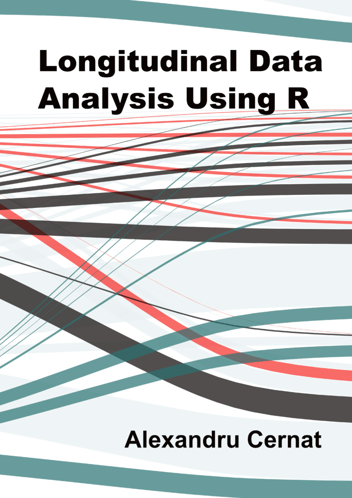
If that was useful you might also like the Longitudinal Data Analysis Using R book.
This covers everything you need to work with longitudinal data. It introduces the key concepts related to longitudinal data, the basics of R and regression. It also shows using real data how to prepare, explore and visualize longitudinal data. In addition, it discusses in depth popular statistical models such as the multilevel model for change, the latent growth model and the cross-lagged model.


Great blog! Very clear,
Is there a typo in the formula for the multilevel model in the section where you compare the equation for the two models. You give the formula for the multilevel model as:
Yij = γ00 + γ10TIMEij + ξ0i + ξ1i + ϵij
Should the ξ1i term be multiplied by TIME?
Great catch! Thank you. Now it’s fixed.