Easy way to make a codebook in R

R is one of the most popular packages in the social and data sciences. The fact that it’s open source and incredibly flexible has made it one of the to go tools for statisticians and data scientists. Unfortunately there is also a relative steep learning curve compared to traditional software such as SPSS and Stata. One thing that newly “converted” R users miss is a way to see a description of all the variables in the data. For example, in SPSS you could easily see the variables codes, labels, missing codes, etc. While there is no off the shelf way to get the equivalent it is very easy to create a codebook in R. This is just an example how you could do one in just a few lines.

We will use two packages. We will use haven to import data saved in other formats, such as from SPSS or Stata. The advantage of such data formats is that it has information about the variables stored within. We will also use tidyverse which is a collection of packages that is useful for cleaning data.

As an example I will be importing wave 7 of the European Social Survey. This is a freely available data that includes tens of countries and hundred of very interesting questions. You can download it from here: https://www.europeansocialsurvey.org/

I import the Stata version as this has the labels we want (other formats, like SPSS, also work). Other types of data, such as “csv” or “tsv”, do not have labels so you might need to find an alternative way to get that info when only those are available.

# import data with labels from the "data" folder
df <- read_dta("./data/ESS7e02_1.dta")

df

## # A tibble: 40,185 x 601
##    name  essround edition proddate  idno cntry   tvtot   tvpol ppltrst  pplfair
##    <chr>    <dbl> <chr>   <chr>    <dbl> <chr> <dbl+l> <dbl+l> <dbl+l> <dbl+lb>
##  1 ESS7~        7 2.1     01.12.2~     1 AT    4 [Mor~ 1 [Les~ 7 [7]    7 [7]  
##  2 ESS7~        7 2.1     01.12.2~     2 AT    7 [Mor~ 3 [Mor~ 5 [5]    5 [5]  
##  3 ESS7~        7 2.1     01.12.2~     3 AT    6 [Mor~ 2 [0,5~ 6 [6]    8 [8]  
##  4 ESS7~        7 2.1     01.12.2~     4 AT    3 [Mor~ 1 [Les~ 5 [5]    3 [3]  
##  5 ESS7~        7 2.1     01.12.2~     5 AT    2 [0,5~ 2 [0,5~ 3 [3]    7 [7]  
##  6 ESS7~        7 2.1     01.12.2~     6 AT    2 [0,5~ 2 [0,5~ 0 [You~ 10 [Mos~
##  7 ESS7~        7 2.1     01.12.2~     7 AT    7 [Mor~ 5 [Mor~ 5 [5]    6 [6]  
##  8 ESS7~        7 2.1     01.12.2~    13 AT    3 [Mor~ 1 [Les~ 5 [5]    7 [7]  
##  9 ESS7~        7 2.1     01.12.2~    14 AT    4 [Mor~ 1 [Les~ 9 [9]    6 [6]  
## 10 ESS7~        7 2.1     01.12.2~    21 AT    5 [Mor~ 2 [0,5~ 5 [5]    4 [4]  
## # ... with 40,175 more rows, and 591 more variables: pplhlp <dbl+lbl>,
## #   polintr <dbl+lbl>, psppsgv <dbl+lbl>, actrolg <dbl+lbl>, psppipl <dbl+lbl>,
## #   cptppol <dbl+lbl>, ptcpplt <dbl+lbl>, etapapl <dbl+lbl>, trstprl <dbl+lbl>,
## #   trstlgl <dbl+lbl>, trstplc <dbl+lbl>, trstplt <dbl+lbl>, trstprt <dbl+lbl>,
## #   trstep <dbl+lbl>, trstun <dbl+lbl>, vote <dbl+lbl>, prtvtbat <dbl+lbl>,
## #   prtvtcbe <dbl+lbl>, prtvtech <dbl+lbl>, prtvtdcz <dbl+lbl>,
## #   prtvede1 <dbl+lbl>, prtvede2 <dbl+lbl>, prtvtcdk <dbl+lbl>,
## #   prtvteee <dbl+lbl>, prtvtces <dbl+lbl>, prtvtcfi <dbl+lbl>,
## #   prtvtcfr <dbl+lbl>, prtvtbgb <dbl+lbl>, prtvtehu <dbl+lbl>,
## #   prtvtaie <dbl+lbl>, prtvtcil <dbl+lbl>, prtvalt1 <dbl+lbl>,
## #   prtvalt2 <dbl+lbl>, prtvalt3 <dbl+lbl>, prtvtfnl <dbl+lbl>,
## #   prtvtbno <dbl+lbl>, prtvtcpl <dbl+lbl>, prtvtbpt <dbl+lbl>,
## #   prtvtbse <dbl+lbl>, prtvtesi <dbl+lbl>, contplt <dbl+lbl>,
## #   wrkprty <dbl+lbl>, wrkorg <dbl+lbl>, badge <dbl+lbl>, sgnptit <dbl+lbl>,
## #   pbldmn <dbl+lbl>, bctprd <dbl+lbl>, clsprty <dbl+lbl>, prtclcat <dbl+lbl>,
## #   prtclcbe <dbl+lbl>, prtclech <dbl+lbl>, prtcldcz <dbl+lbl>,
## #   prtclede <dbl+lbl>, prtclcdk <dbl+lbl>, prtcleee <dbl+lbl>,
## #   prtcldes <dbl+lbl>, prtclcfi <dbl+lbl>, prtclcfr <dbl+lbl>,
## #   prtclbgb <dbl+lbl>, prtclehu <dbl+lbl>, prtclaie <dbl+lbl>,
## #   prtcldil <dbl+lbl>, prtclalt <dbl+lbl>, prtclenl <dbl+lbl>,
## #   prtclbno <dbl+lbl>, prtclfpl <dbl+lbl>, prtcldpt <dbl+lbl>,
## #   prtclbse <dbl+lbl>, prtclesi <dbl+lbl>, prtdgcl <dbl+lbl>,
## #   lrscale <dbl+lbl>, stflife <dbl+lbl>, stfeco <dbl+lbl>, stfgov <dbl+lbl>,
## #   stfdem <dbl+lbl>, stfedu <dbl+lbl>, stfhlth <dbl+lbl>, gincdif <dbl+lbl>,
## #   freehms <dbl+lbl>, euftf <dbl+lbl>, imsmetn <dbl+lbl>, imdfetn <dbl+lbl>,
## #   eimpcnt <dbl+lbl>, impcntr <dbl+lbl>, imbgeco <dbl+lbl>, imueclt <dbl+lbl>,
## #   imwbcnt <dbl+lbl>, happy <dbl+lbl>, sclmeet <dbl+lbl>, inprdsc <dbl+lbl>,
## #   sclact <dbl+lbl>, crmvct <dbl+lbl>, aesfdrk <dbl+lbl>, health <dbl+lbl>,
## #   hlthhmp <dbl+lbl>, rlgblg <dbl+lbl>, rlgdnm <dbl+lbl>, rlgdnbat <dbl+lbl>,
## #   rlgdnbe <dbl+lbl>, rlgdnach <dbl+lbl>, ...

We see it’s a moderately large dataset with around 40,000 cases and 600 variables. Quite hard to do a codebook by hand!

Let’s check if it imported the attributes. We will use the attributes() command on the “tvtot” variable.

# let's see attributes for tvtot variable
attributes(df$tvtot)

## $label
## [1] "TV watching, total time on average weekday"
## 
## $format.stata
## [1] "%10.0g"
## 
## $class
## [1] "haven_labelled" "vctrs_vctr"     "double"        
## 
## $labels
##                     No time at all                 Less than 0,5 hour 
##                                  0                                  1 
##                 0,5 hour to 1 hour  More than 1 hour, up to 1,5 hours 
##                                  2                                  3 
## More than 1,5 hours, up to 2 hours More than 2 hours, up to 2,5 hours 
##                                  4                                  5 
## More than 2,5 hours, up to 3 hours                  More than 3 hours 
##                                  6                                  7 
##                            Refusal                         Don't know 
##                                 77                                 88 
##                          No answer 
##                                 99

It seems it has what we want. Here we will concentrate on extracting the “label” information. This can be extracted using this code:

attributes(df$tvtot)$label

## [1] "TV watching, total time on average weekday"

We don’t want to do this by hand for hundreds of variables so we need to use some programming skills to automate this. We will us the map() function which is similar in spirit to a loop but it is more efficient in R (it’s similar to sapply()). This loops through all the variables of a dataset and applies a function. So, in turn, each variable becomes x and then applies the function we want. In this case we simply apply the function that extracts the label attribute.

Here we use a specific version of map which creates a dataset (map_df()). Because this is in the wide format, having 600 variables and one row, we reshape it using the gather() command. So all together this is how the command looks like:

# let the magic happen
codebook <- map_df(df, function(x) attributes(x)$label) %>% 
  gather(key = Code, value = Label)

# look at it
codebook

## # A tibble: 601 x 2
##    Code     Label                                                        
##    <chr>    <chr>                                                        
##  1 name     Title of dataset                                             
##  2 essround ESS round                                                    
##  3 edition  Edition                                                      
##  4 proddate Production date                                              
##  5 idno     Respondent's identification number                           
##  6 cntry    Country                                                      
##  7 tvtot    TV watching, total time on average weekday                   
##  8 tvpol    TV watching, news/politics/current affairs on average weekday
##  9 ppltrst  Most people can be trusted or you can't be too careful       
## 10 pplfair  Most people try to take advantage of you, or try to be fair  
## # ... with 591 more rows

Two lines for a codebook! This is pretty nifty, we already have a decent looking codebook but we can use this trick to add more information. So lets say we want to know what type of variable it is, the average (if it can be calculated) and the proportion of missing cases. We can combine our new knowledge of map() with some other functions. So, for example, typeof() tells us what kind of variable we have. Similarly, mean(na.rm = T) gives us the average (the na.rm = T means “ignore missing cases”).

Finally, we combine the map(), mean() and is.na() commands to find out the proportion of missing cases. We start by using is.na() which checks if each case is missing. For each case it gives us a TRUE if it is missing, or a FALSE if it’s not missing. If we calculate the average of this new variable TRUE will become 1 and FALSE will become 0. The average of this will give us the proportion of missing cases.

You will also notice that we use slightly different versions of map(). We can tell R what kind of object to create in this way. For example, map_chr() tells R to make the result of the function a string vector while map_dbl() creates a numeric vector.

# get more info
codebook <- codebook %>% 
  mutate(Type = map_chr(df, typeof),
         Mean = map_dbl(df, mean, na.rm = T),
         Prop_miss = map_dbl(df, function(x) mean(is.na(x)))) 

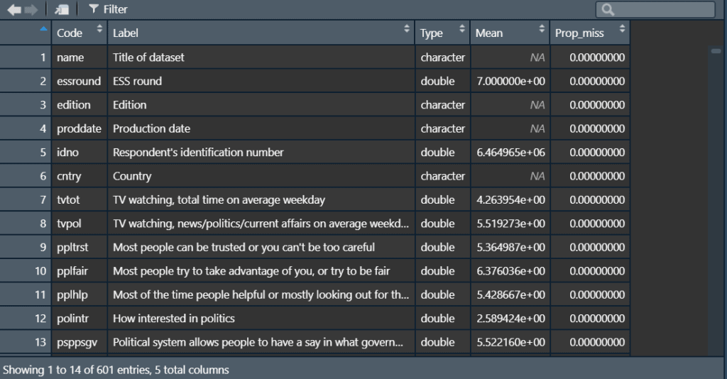
codebook

## # A tibble: 601 x 5
##    Code    Label                                     Type         Mean Prop_miss
##    <chr>   <chr>                                     <chr>       <dbl>     <dbl>
##  1 name    Title of dataset                          charact~  NA              0
##  2 essrou~ ESS round                                 double     7.00e0         0
##  3 edition Edition                                   charact~  NA              0
##  4 prodda~ Production date                           charact~  NA              0
##  5 idno    Respondent's identification number        double     6.46e6         0
##  6 cntry   Country                                   charact~  NA              0
##  7 tvtot   TV watching, total time on average weekd~ double     4.26e0         0
##  8 tvpol   TV watching, news/politics/current affai~ double     5.52e0         0
##  9 ppltrst Most people can be trusted or you can't ~ double     5.36e0         0
## 10 pplfair Most people try to take advantage of you~ double     6.38e0         0
## # ... with 591 more rows

In R you can also see the data in a nicer way that is also easy to search using View().

# for searchable view
View(codebook)

Finally, we can save this for future use. Now we can also use something easy to transfer such as a “csv” format. Here we save it in a sub-folder called “data”.

write_csv(codebook, "./data/codebook.csv")

Hope this is useful. In general, if you can, try to download data that has such information as labels. Often you can do this on websites like the UK Data Archive. This makes it possible to extract the labels one way or another to make your work with data easier.