In previous posts we have introduced the multilevel model for change, a powerful model that can be used to estimate change in time while separating within and between variation. While we discussed the basic model in some detail it can be expanded in a couple of different ways. Here we will cover how we can estimate non-linear change in time using the multilevel framework.
In the basic multilevel model for change we have only one coefficient to describe the effect of time. This implies a stable or linear rate of change. In many applications this is not an appropriate assumption as rates of change can be different at different points in time. There are two main ways of modeling these non-linear trends: including polynomials and treating time as discrete.
Nolinear change in time using polynomials
Let’s start with the first approach, including polynomials of time in the model. This is easily done by creating new variables that take the values of time and square/cube/etc them. We will use as reference “wave0” which is a recoded version of time that starts from 0 (this is used to make the intercept easier to interpret, as discussed here).
usl <- mutate(usl,
              wave0 = wave - 1,
              wave_sq = wave0^2,
              wave_cu = wave0^3)

select(usl, wave0, wave_sq, wave_cu)
## # A tibble: 52,512 × 3
## wave0 wave_sq wave_cu
## <dbl> <dbl> <dbl>
## 1 0 0 0
## 2 1 1 1
## 3 2 4 8
## 4 3 9 27
## 5 4 16 64
## 6 5 25 125
## 7 0 0 0
## 8 1 1 1
## 9 2 4 8
## 10 3 9 27
## # … with 52,502 more rows
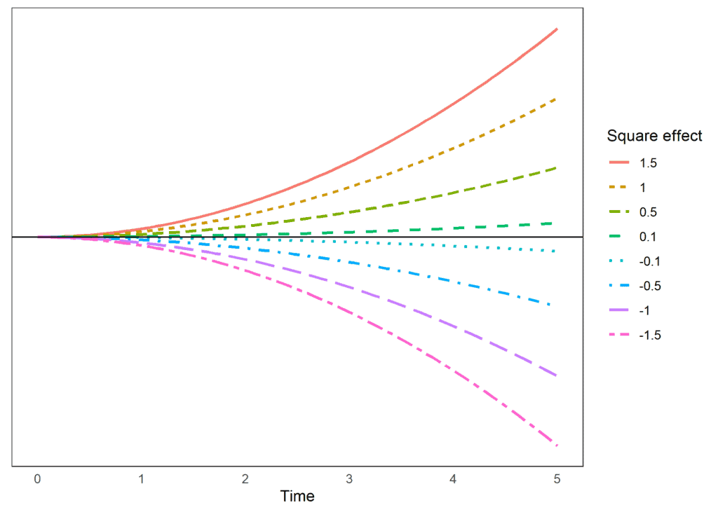
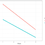
By including in a model these new variables we allow for the effect of time to shift. When time has low values the main effect will have a large impact on the outcome, as time increases the square and the cube will become more and more important (due to their increased size). This allows for the rate of change to be different at different points in time. With the addition of each polynomial we allow for the rate of change to “bend” once. If the effect of the polynomial is positive, the bend will be upwards, if it’s negative, it will bend downwards. The larger the size the stronger the shift. Let’s look at an example. Below are the predicted scores for a hypothetical outcome where the main effect is 0. We see how the size of the outcome changes in time non-linearly due to the effect of the square estimate:
We can also look at some hypothetical examples that include a cube effect as well. Again, the main effect is 0, so it would indicate no trend. But the combination of square and cube effects allows for different types of trends in time.
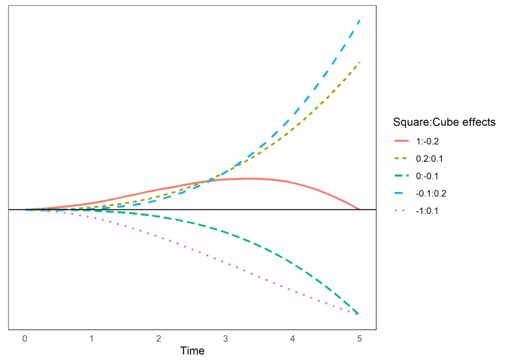
If we look at the situation when the square effect is 1 and the cube has an effect of -0.2 we see an initial upward trend and then a decrease, reaching 0 by wave 5. If both the square and the cube are positive we have an accelerated trend that increases as time passes. We also see that we can reach similar estimates in wave 5 with different change patterns. For example, both having a square effect of -1 and a cube effect of 0.1 and having a square effect of 0 and a cube effect of -.1 reach a similar point in wave 5 but if we would continue that trend the trajectories would become quite different.
Let’s look at the linear model so we can use it as a reference (for an in depth interpretation of the coefficient check this post).
m2 <- lmer(data = usl, logincome ~ 1 + wave0 +
              (1 + wave0 | pidp))

summary(m2)
## Linear mixed model fit by REML ['lmerMod']
## Formula: logincome ~ 1 + wave0 + (1 + wave0 | pidp)
## Data: usl
##
## REML criterion at convergence: 98116.1
##
## Scaled residuals:
## Min 1Q Median 3Q Max
## -7.8825 -0.2306 0.0464 0.3206 5.8611
##
## Random effects:
## Groups Name Variance Std.Dev. Corr
## pidp (Intercept) 0.69590 0.8342
## wave0 0.01394 0.1181 -0.51
## Residual 0.21052 0.4588
## Number of obs: 52512, groups: pidp, 8752
##
## Fixed effects:
## Estimate Std. Error t value
## (Intercept) 7.057963 0.009598 735.39
## wave0 0.041934 0.001723 24.34
These results imply that income is increasing linearly by 0.04 each wave. If we believe there are non-linear effects we can add the polynomials to the model. For example, we can include the square effect using this code:
m2_sq <- lmer(data = usl, logincome ~ 1 + wave0 + wave_sq +
              (1 + wave0 | pidp))

summary(m2_sq)
## Linear mixed model fit by REML ['lmerMod']
## Formula: logincome ~ 1 + wave0 + wave_sq + (1 + wave0 | pidp)
## Data: usl
##
## REML criterion at convergence: 98073.4
##
## Scaled residuals:
## Min 1Q Median 3Q Max
## -7.9234 -0.2301 0.0478 0.3199 5.8314
##
## Random effects:
## Groups Name Variance Std.Dev. Corr
## pidp (Intercept) 0.69607 0.8343
## wave0 0.01396 0.1182 -0.51
## Residual 0.21019 0.4585
## Number of obs: 52512, groups: pidp, 8752
##
## Fixed effects:
## Estimate Std. Error t value
## (Intercept) 7.0381081 0.0099629 706.428
## wave0 0.0717158 0.0043647 16.431
## wave_sq -0.0059563 0.0008021 -7.426
Looking at the fixed effects for the linear and the square of time we observe an initial positive slope (0.07) followed by a negative square effect (-0.01). As such, we would expect an initial increase in logincome and then a decrease.
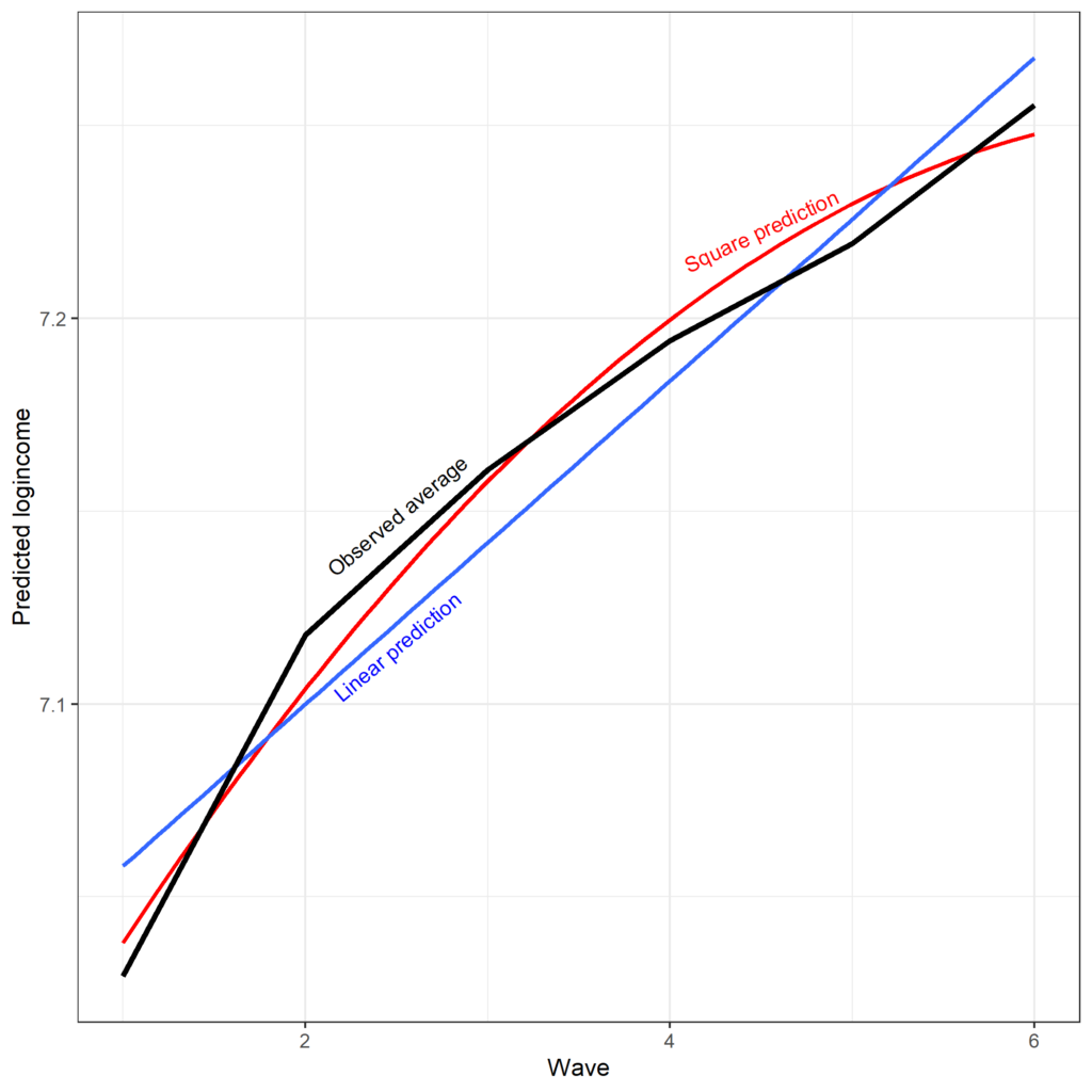
We can also compare the predicted scores from the model that assumes linear change and the model that also includes square effects versus the observed average. It appears that square effect fits better the observed data albeit not perfectly.
One thing to note about the previous non-linear model is that we did not include the square effect in the random part of the model. This means that we assume that the non-linear bend in time is the same for everyone. We can free that assumption by including the square time in the random part of the model, thus allowing each individual to have their own non-linear trend. While this is typically a more realistic assumption this model can be complex and lead to estimation issues, depending on the outcome and the number of cases and waves. For example, this model does not work for our current data but would estimate if we used 11 waves of data.
m2_sq_re <- lmer(data = usl_all, logincome ~ 1 + wave0 + wave_sq +
              (1 + wave0 + wave_sq | pidp))
summary(m2_sq_re)
## Linear mixed model fit by REML ['lmerMod']
## Formula: logincome ~ 1 + wave0 + wave_sq + (1 + wave0 + wave_sq | pidp)
## Data: usl_all
##
## REML criterion at convergence: 883956.3
##
## Scaled residuals:
## Min 1Q Median 3Q Max
## -7.0310 -0.1406 0.0725 0.2895 5.5940
##
## Random effects:
## Groups Name Variance Std.Dev. Corr
## pidp (Intercept) 1.6890306 1.29963
## wave0 0.0987768 0.31429 -0.63
## wave_sq 0.0007027 0.02651 0.43 -0.92
## Residual 0.6234185 0.78957
## Number of obs: 306953, groups: pidp, 50994
##
## Fixed effects:
## Estimate Std. Error t value
## (Intercept) 6.6498507 0.0064688 1027.98
## wave0 0.1218175 0.0022977 53.02
## wave_sq -0.0079053 0.0002277 -34.72
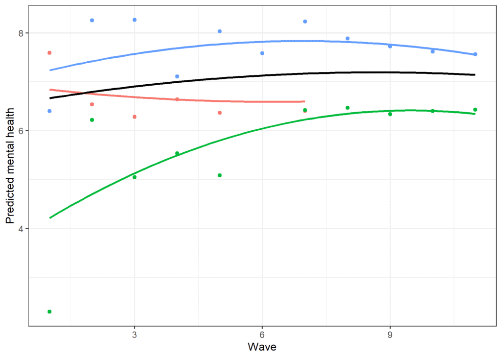
We observe again an initial positive trend and then a negative square effect when we use 11 waves as when we analyzed only 4. If we sample a few cases and plot the predicted scores we can see the model implied trends and capture some of the individual variation present due to the random effect for the square effect.
An alternative way to model non-linear change is to treat time as a discrete variable. In that case we can estimate the expected value of the outcome at each point in time or in a particular range of time. The most general approach is to treat each time point as a discrete variable. While this doesn’t make any assumptions about the shape of the change in time it is a complex model that may have estimation problems.
To try this out with our model we can define the time variable as a factor. By default lmer() (like the lm() command) transforms factors in dummy variables and treats the first category as the reference. We can use this to model non-linear change.
usl <- mutate(usl,
              wave_fct = as.factor(wave))
We can now include this in our model.
m2_dummy <- lmer(data = usl, logincome ~ 1 + wave_fct +
                   (1 + wave0 | pidp))

summary(m2_dummy)
## Linear mixed model fit by REML ['lmerMod']
## Formula: logincome ~ 1 + wave_fct + (1 + wave0 | pidp)
## Data: usl
##
## REML criterion at convergence: 98071.9
##
## Scaled residuals:
## Min 1Q Median 3Q Max
## -7.9319 -0.2313 0.0482 0.3210 5.8448
##
## Random effects:
## Groups Name Variance Std.Dev. Corr
## pidp (Intercept) 0.69611 0.8343
## wave0 0.01397 0.1182 -0.51
## Residual 0.21009 0.4584
## Number of obs: 52512, groups: pidp, 8752
##
## Fixed effects:
## Estimate Std. Error t value
## (Intercept) 7.029381 0.010176 690.81
## wave_fct2 0.088438 0.007043 12.56
## wave_fct3 0.131348 0.007375 17.81
## wave_fct4 0.164791 0.007898 20.86
## wave_fct5 0.190032 0.008576 22.16
## wave_fct6 0.225894 0.009376 24.09
Notice that we treat the random part of the model still linearly. Again, estimating a random effect at each wave can lead to issues with model estimation so we use a simplified random effect.
Using this model we can calculate the expected mental health at each point in time. The intercept again refers to the expected value at the beginning of the study as that is the reference or missing category. The expected value is 7.03. To get the expected value for wave two we add the intercept and the effect of wave 2: 7.03 + 0.09 = 7.11. We can use a similar approach for waves 3 and 4. We can also compare the results from this model with the observed scores and the predictions from the square model.
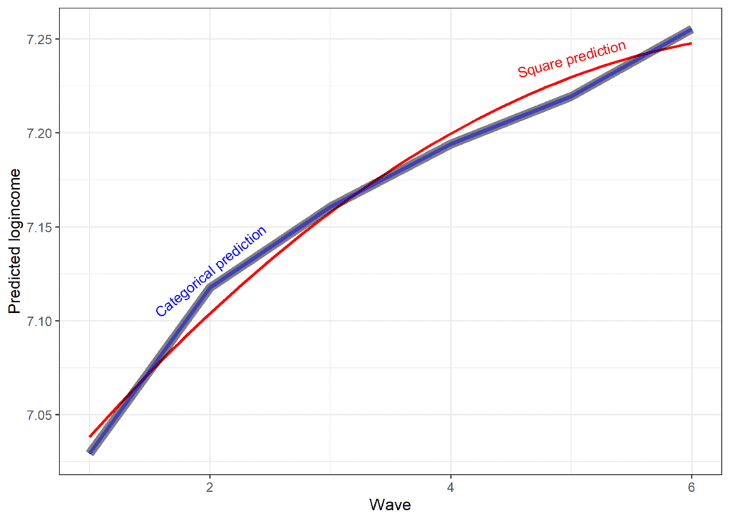
We see that the new prediction is almost identical to the observed data (lines overlap). That being said there is a trade-off between the simplicity of the model and how well it explains the data. We can formally compare the different models we estimated to decide how to treat the change in time for logincome.
anova(m2, m2_sq, m2_dummy)## Data: usl
## Models:
## m2: logincome ~ 1 + wave0 + (1 + wave0 | pidp)
## m2_sq: logincome ~ 1 + wave0 + wave_sq + (1 + wave0 | pidp)
## m2_dummy: logincome ~ 1 + wave_fct + (1 + wave | pidp)
## npar AIC BIC logLik deviance Chisq Df Pr(>Chisq)
## m2 6 98109 98163 -49049 98097
## m2_sq 7 98056 98118 -49021 98042 55.108 1 1.141e-13 ***
## m2_dummy 10 98043 98131 -49011 98023 19.629 3 0.0002026 ***
## ---
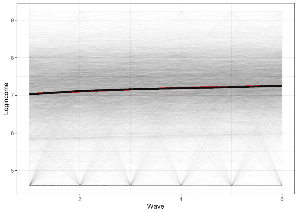
## Signif. codes: 0 '***' 0.001 '**' 0.01 '*' 0.05 '.' 0.1 ' ' 1Based on the AIC and the Chi square we should select the final model, where we treat time as categorical while based on BIC we should select the model using square effects. The graph below shows that while the square effect (red line) does not perfectly represent the true average (black line) it is relatively close given the amount of variability in the data (the thin lines represent the scores of different individuals).
Conclusions
Hopefully this gives you an idea about how the multilevel model for change can be expanded to include non-linear effects. Other, more complex trends, can be estimated using models such as splines (an introduction here). The model can also be extended to include time constant predisctors as discussed here. You can also compare this approach with modeling non-linear effects using Latent Growth Models.
If that was useful you might also like the Longitudinal Data Analysis Using R book.
This covers everything you need to work with longitudinal data. It introduces the key concepts related to longitudinal data, the basics of R and regression. It also shows using real data how to prepare, explore and visualize longitudinal data. In addition, it discusses in depth popular statistical models such as the multilevel model for change, the latent growth model and the cross-lagged model.
More blog posts
 Explaining change in time using multilevel models and time constant predictors
 Summer schools in applied statistics and survey methodology 2023
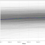 Estimating non-linear change with Latent Growth Models in R
 Estimating and visualizing change in time using Latent Growth Models with R
 Interview for Frontmatter podcast discussing survey research and longitudinal data analysis
 Understanding causal direction using the cross-lagged model
Pingback: Understanding causal direction using the cross-lagged model - Alexandru Cernat
Pingback: Explaining change in time using multilevel models and time constant predictors - Alexandru Cernat
Pingback: Estimating multilevel models for change in R - Alexandru Cernat