In previous posts we discussed the multilevel model for change, a way of investigating average change in time while accounting for individual level variation. In this blog post we will discuss how to extend this model to include predictors.
Time varying versus time constant variables
When working with longitudinal data we can consider variables either as time varying or as time constant. For example, a survey measure of general satisfaction is a time varying variable as it is collected in each wave. So, for each individual this could change (although it does not have to change). The year of birth is a time constant variable. It is enough to collect this information once from each individual as we do not expect it to change.
There are also some situations where we have a choice to treat a variable as time constant or time varying. For example, we could recode birth year as age, which is a time varying variable. Similarly, we could take the average of general satisfaction for each individual and make that variable time constant. In such situations the decision to treat a variable as time constant or variable should be based on theoretical considerations, our data and on the modelling strategy used.
Explaining Change
Here we will discuss how we can expand the multilevel model to include time constant predictors. In a previous post we explored how best to describe the change in time of the outcome by including non-linear effects. This is an important first step in analyzing longitudinal data. Nevertheless, often we want to understand the causes of that change or at least how different groups may have different rates of change. We will turn now to this aspect, discussing the inclusion of time constant predictors
Including Time Constant Predictors
We will start by adding a time constant predictor to our model. As an example, let’s explore how the change in mental health is different for men and women (where we treat these as time constant). If we add the “gndr” variable to our model the new formula for our regression will be:
Yij = γ00 + γ01GNDRi + γ10TIMEij + ξ0i + ξ1iTIMEij + ϵij
The interpretation of the coefficients is mostly the same as before. The interpretation of the intercept (γ00) changes and now refers to the expected value of the outcome when “gndr” and “time” are 0. In our case this would refer to males at the beginning of the study. The effect of “gndr” (γ10) refers how different are females to males in their mental health. The interpretation of the random effects is the same as before.
To keep things simple we will use the linear change in time model but this can be easily expanded to include non-linear change.
Let’s run this model:
m3 <- lmer(data = usl, sf12mcs ~ 1 + wave0 + gndr +
             (1 + wave0 | pidp))
summary(m3)
## Linear mixed model fit by REML ['lmerMod'] ## Formula: sf12mcs ~ 1 + wave0 + gndr + (1 + wave0 | pidp) ## Data: usl ## ## REML criterion at convergence: 669722 ## ## Scaled residuals: ## Min 1Q Median 3Q Max ## -6.0382 -0.4070 0.1166 0.5036 4.6337 ## ## Random effects: ## Groups Name Variance Std.Dev. Corr ## pidp (Intercept) 52.552 7.249 ## wave0 2.915 1.707 -0.25 ## Residual 40.841 6.391 ## Number of obs: 94435, groups: pidp, 26769 ## ## Fixed effects: ## Estimate Std. Error t value ## (Intercept) 51.71612 0.07857 658.22 ## wave0 -0.41987 0.02139 -19.63 ## gndrFemale -1.96590 0.09727 -20.21 ## ## Correlation of Fixed Effects: ## (Intr) wave0 ## wave0 -0.365 ## gndrFemale -0.700 -0.001
We will concentrate on interpreting the fixed part of the model. As mentioned before, the intercept (51.72) represents the expected mental health at the beginning of the study. The effect of “wave0” (-0.42) refers to rate of change in mental health, as before. This effect is the same both for men and women. Finally, the effect of “gndr” (-1.97) indicates how females are different to men or mental health. In our data it appears that they have lower mental health on average.
This model can be easily expanded to include multiple time constant predictors of different nature, categorical or continuous. The interpretation will be the same as in a regular regression.
Allowing for different rates of change
One important assumption we made so far is that the rate of change is the same for men and females. That means that the difference in mental state remains constant in time. This is often an important question that we want to explore. From a substantive point of view having different rates of change, which would lead to convergence or divergence, is very important. To explicitly explore this in our model we can add an interaction between gender and time. This would allow for different rates of change for men and women. We would write this model as:
Yij = γ00 + γ01GNDRi + γ10TIMEij + γ11GNDRi * TIMEij + ξ0i + ξ1iTIMEij + ϵij
We can easily include interactions in lmer() by adding the two variables separated by :. So our new model is:
m4 <- lmer(data = usl, sf12mcs ~ 1 + wave0 + gndr + gndr:wave0 +
             (1 + wave0 | pidp))
summary(m4)
## Linear mixed model fit by REML ['lmerMod'] ## Formula: sf12mcs ~ 1 + wave0 + gndr + gndr:wave0 + (1 + wave0 | pidp) ## Data: usl ## ## REML criterion at convergence: 669726.4 ## ## Scaled residuals: ## Min 1Q Median 3Q Max ## -6.0380 -0.4067 0.1166 0.5035 4.6335 ## ## Random effects: ## Groups Name Variance Std.Dev. Corr ## pidp (Intercept) 52.551 7.249 ## wave0 2.915 1.707 -0.25 ## Residual 40.841 6.391 ## Number of obs: 94435, groups: pidp, 26769 ## ## Fixed effects: ## Estimate Std. Error t value ## (Intercept) 51.710221 0.085255 606.535 ## wave0 -0.415472 0.032649 -12.726 ## gndrFemale -1.955542 0.113295 -17.261 ## wave0:gndrFemale -0.007702 0.043216 -0.178 ## ## Correlation of Fixed Effects: ## (Intr) wave0 gndrFm ## wave0 -0.514 ## gndrFemale -0.753 0.387 ## wv0:gndrFml 0.388 -0.755 -0.513 ## optimizer (nloptwrap) convergence code: 0 (OK) ## Model failed to converge with max|grad| = 0.00590502 (tol = 0.002, component 1)
When we have interactions in a regression model we have to be careful how we interpret the main effects as well. In our results the interpretation of the intercept stays the same (the expected value at the beginning of the study for men is 51.71) but the interpretation of the other coefficients is different. The effect of time (-0.42) refers now to the rate of change in mental health for men and the effect of gender (-1.96) now refers to the difference in mental health at the beginning of the study. These two interpretations are due to the interaction effect that we now have in our model. This final coefficient (-0.008) can be interpreted as how different is the rate of change for females compared to men. To get an exact size we can get the rate of change for men (-0.42) and add it to the interaction effect (-0.008) leading to a rate of change for females of (-0.4234715). This would indicate that mental health is deteriorating at a slightly lower pace for females compared to men. Given that females start out with lower mental health (-1.96) this implies that in time the two will converge. That being said the effect of the interaction is quite small so it would take a long time for the two to converge.
We can also see this visually by using the predicted scores:
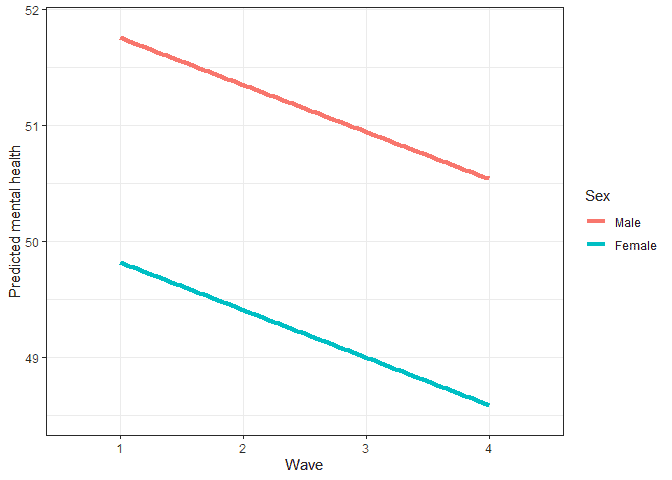
We see that men start with higher mental health with values in line to the intercept. The two lines showing the change in time for men and female look almost parallel, highlighting the fact that the interaction effect is quite small here.
We can expand the model to see a more clear example of convergence. Below we include the effect of degree, another variable we treat as time constant, as well as the interaction with time. We keep the main effect of sex but exclude the interaction with time given the small effect.
m5 <- lmer(data = usl, sf12mcs ~ 1 + wave0 + gndr +
             degree + degree:wave0 +
             (1 + wave0 | pidp))
summary(m5)
## Linear mixed model fit by REML ['lmerMod'] ## Formula: sf12mcs ~ 1 + wave0 + gndr + degree + degree:wave0 + (1 + wave0 | ## pidp) ## Data: usl ## ## REML criterion at convergence: 669330.5 ## ## Scaled residuals: ## Min 1Q Median 3Q Max ## -6.0343 -0.4070 0.1157 0.5045 4.6426 ## ## Random effects: ## Groups Name Variance Std.Dev. Corr ## pidp (Intercept) 52.35 7.236 ## wave0 2.91 1.706 -0.25 ## Residual 40.83 6.390 ## Number of obs: 94391, groups: pidp, 26751 ## ## Fixed effects: ## Estimate Std. Error t value ## (Intercept) 52.34373 0.10892 480.580 ## wave0 -0.50243 0.03546 -14.170 ## gndrFemale -1.96869 0.09720 -20.255 ## degreeNo degree -0.97285 0.11714 -8.305 ## wave0:degreeNo degree 0.12863 0.04446 2.893 ## ## Correlation of Fixed Effects: ## (Intr) wave0 gndrFm dgrNdg ## wave0 -0.443 ## gndrFemale -0.505 -0.001 ## degreeNdegr -0.693 0.412 0.001 ## wv0:dgrNdgr 0.353 -0.798 0.000 -0.513 ## optimizer (nloptwrap) convergence code: 0 (OK) ## Model failed to converge with max|grad| = 0.0233356 (tol = 0.002, component 1)
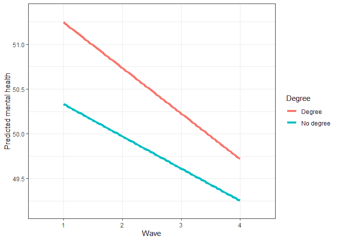
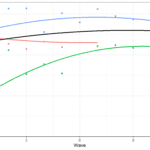
Now the intercept (52.34) refers to the expected mental health in wave 1 for men with a degree. At the beginning of the study it appears that participants without a degree have lower levels of mental health (-0.97). And while mental health is deteriorating with the passage of each wave (-0.5) this is happening at a lower rate for those without a degree (0.13), again implying a convergence. Again, we can use the predicted scores to see this more clearly in a graph:
Conclusions
The multilevel model for change can be easily expanded to include time constant predictors. For the most part the interpretation is similar to that from multiple regressions. When including interactions with time, to allow for different rates of change for subgroup, care is needed with the interpretations. You have seen above some example code of ow you can use predicted scores and visualizations to better understand the results of your model.
If that was useful you might also like the Longitudinal Data Analysis Using R book.
This covers everything you need to work with longitudinal data. It introduces the key concepts related to longitudinal data, the basics of R and regression. It also shows using real data how to prepare, explore and visualize longitudinal data. In addition, it discusses in depth popular statistical models such as the multilevel model for change, the latent growth model and the cross-lagged model.
More blog posts
 Estimating non-linear change in time using the multilevel model for change
 Summer schools in applied statistics and survey methodology 2023
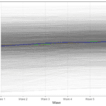 Estimating non-linear change with Latent Growth Models in R
 Estimating and visualizing change in time using Latent Growth Models with R
 Interview for Frontmatter podcast discussing survey research and longitudinal data analysis
 Understanding causal direction using the cross-lagged model
Pingback: Estimating non-linear change in time using the multilevel model for change - Alexandru Cernat
Pingback: Estimating multilevel models for change in R - Alexandru Cernat