Longitudinal data is essential for understanding how individuals, organizations and societies change. But what exactly is longitudinal data? How do we create, store and reshape such data to answer our research questions?
What is longitudinal data?
Different academic fields have different definitions of longitudinal data. To investigate individual level change and apply the methods often discussed in this blog longitudinal data needs to meet one important criteria: data has to be collected multiple times from the same elements. Elements can be individuals, organizations, societies, sensors and so on. This definition is not met by designs such as repeated cross-sectional studies (where there are new individuals each wave) but is met by designs such as panels studies (where the same individuals are interviewed regularly). This definition covers a wide range of other data sources such as administrative data and sensor data.
Types of variables
Before we discuss how to create and store longitudinal data it is important to understand the different types of variables we can have in this context. When working with longitudinal data we can consider variables either as time varying or as time constant. For example, if we collect a variable such as general satisfaction each wave we can treat it as time varying. As a result, for each individual at each wave this value could change (although it not mandatory). Other variables, that do not change in time, such as year of birth, are treated as time constant variables. It is enough to collect this information once from each individual as we do not expect it to change.
There are also some situations where we can choose if we treat a variable as time constant or time varying. For example, we could recode birth year as age, which is a time varying variable. Similarly, we could take the average of “general satisfaction” for each individual and make that variable time constant. In such situations the decision to treat a variable as time constant or variable should be based on theoretical considerations, the data available and on the modelling strategy used.
Creating longitudinal data
Typically, for larger studies data is stored separately for each wave. For example, after downloading Understanding Society we have one dataset for each wave and each level/type (e.g., individual level data, household level data, relationship data). To do longitudinal data analysis we need to bring these datasets together.
For example, imagine we have these two datasets:
data_w1

## # A tibble: 4 × 3
##   id         sf1 birthy
##   <chr>    <dbl>  <dbl>
## 1 68004087     4   1986
## 2 68008847     2   2001
## 3 68009527     3   1978
## 4 68009521     5   1988

data_w2

## # A tibble: 4 × 2
##   id         sf1
##   <chr>    <dbl>
## 1 68004087     3
## 2 68008847     3
## 3 68009527     3
## 4 68009522     4
To bring the data together we need a unique id for each individual (the “id” column in this case) and we need to decide if variables will be treated as time constant or variable. In this example we can treat “sf1” (a measure of general health) as time variable (it is measured at multiple points in time and can change) while we can treat “birthy” as time constant. The latter is measured just once and does not change in time.
We can then use one of two strategies to merge the data. The first strategy is to merge the datasets by column. There are different commands for this but the ..._join() commands in the “tidyverse” package are very useful here. To bring all the data together we can use full_join() by adding the datasets and the unique id as inputs.
Before we attempt this type of data merging we need to make sure that the time varying variables have unique names. It is usually good practice to add a wave specific suffix:
library(tidyverse)

data_w1b <- rename(data_w1, sf1_1 = sf1)
data_w1b

## # A tibble: 4 × 3
##   id       sf1_1 birthy
##   <chr>    <dbl>  <dbl>
## 1 68004087     4   1986
## 2 68008847     2   2001
## 3 68009527     3   1978
## 4 68009521     5   1988

data_w2b <- rename(data_w2, sf1_2 = sf1)
data_w2b

## # A tibble: 4 × 2
##   id       sf1_2
##   <chr>    <dbl>
## 1 68004087     3
## 2 68008847     3
## 3 68009527     3
## 4 68009522     4
Now we can join the data:
data_w12 <- full_join(data_w1b, data_w2b, by = "id")
data_w12

## # A tibble: 5 × 4
##   id       sf1_1 birthy sf1_2
##   <chr>    <dbl>  <dbl> <dbl>
## 1 68004087     4   1986     3
## 2 68008847     2   2001     3
## 3 68009527     3   1978     3
## 4 68009521     5   1988    NA
## 5 68009522    NA     NA     4
We notice that now we have five individuals in the data and four variables. Three of the individuals are present in both waves while there is an individual that is present in just one of the waves. This could be due to missing data (people dropping out) or new people joining the study.
There are different versions of the ..._join() commands that can facilitate selecting the cases we want. You can find out more here.
The data we created what is known as unbalanced data. This means that we include in the data any case even if it is present just once. If, on the other hand, we wanted to select only cases present in all the waves, also known as balanced data, we could use inner_join():
inner_join(data_w1b, data_w2b, by = "id")

## # A tibble: 3 × 4
##   id       sf1_1 birthy sf1_2
##   <chr>    <dbl>  <dbl> <dbl>
## 1 68004087     4   1986     3
## 2 68008847     2   2001     3
## 3 68009527     3   1978     3
The alternative way to bring data together is to join them by row. Before that it is good practice to create a “time” or “wave” variable so we know where the data comes from.
data_w1c <- mutate(data_w1, wave = 1)
data_w1c

## # A tibble: 4 × 4
##   id         sf1 birthy  wave
##   <chr>    <dbl>  <dbl> <dbl>
## 1 68004087     4   1986     1
## 2 68008847     2   2001     1
## 3 68009527     3   1978     1
## 4 68009521     5   1988     1

data_w2c <- mutate(data_w2, wave = 2)
data_w2c

## # A tibble: 4 × 3
##   id         sf1  wave
##   <chr>    <dbl> <dbl>
## 1 68004087     3     2
## 2 68008847     3     2
## 3 68009527     3     2
## 4 68009522     4     2
We can then use the bind_rows() command to do the merger:
data_l12 <- bind_rows(data_w1c, data_w2c)
data_l12

## # A tibble: 8 × 4
##   id         sf1 birthy  wave
##   <chr>    <dbl>  <dbl> <dbl>
## 1 68004087     4   1986     1
## 2 68008847     2   2001     1
## 3 68009527     3   1978     1
## 4 68009521     5   1988     1
## 5 68004087     3     NA     2
## 6 68008847     3     NA     2
## 7 68009527     3     NA     2
## 8 68009522     4     NA     2
Notice that because the time constant variable is present only in wave 1 it only has missing information in the second one (NA). We could copy the values from the first wave to all the others by first grouping the data by individual and then taking the maximum of the variable:
data_l12 %>%
  group_by(id) %>%
  mutate(birthy = max(birthy, na.rm = T))

## # A tibble: 8 × 4
## # Groups:   id [5]
##   id         sf1 birthy  wave
##   <chr>    <dbl>  <dbl> <dbl>
## 1 68004087     4   1986     1
## 2 68008847     2   2001     1
## 3 68009527     3   1978     1
## 4 68009521     5   1988     1
## 5 68004087     3   1986     2
## 6 68008847     3   2001     2
## 7 68009527     3   1978     2
## 8 68009522     4   -Inf     2
Notice that one individual has -Inf because they have no information available (they joined the study in wave 2).
Which strategy to use when merging longitudinal data? My general recommendation is to use the first approach where we merge by adding columns (also know as mutating joins). One reason is that it gives more control regarding which cases to include in the data. It also makes it easier to identify errors and understand the patterns of participation. Finally, in large datasets we tend to have a mix of time constant and time varying variables. The merger by rows can be complicated in such situations.
Data structures
The two different strategies for merging longitudinal data highlight also that such data can be stored in two different ways: the wide format and the long format. Merging the columns leads to the wide format. Here is another example with four waves:
## # A tibble: 3 × 6
##   id       sf1_1 sf1_2 sf1_3 sf1_4 birthy
##   <chr>    <dbl> <dbl> <dbl> <dbl>  <dbl>
## 1 68004087     4     3     3     4   1986
## 2 68008847     2     3     4     1   2001
## 3 68009527     3     3     3     3   1978
We see that this is similar to cross-sectional data because each row represents data for an individual (with a unique “id”). If we have information from multiple waves it appears as different columns. So, for example “sf1” is measured four times here. The suffix after “_” representing the wave in which the data was collected. We can also have time constant variables that do not have the suffix (like birth year: “birthy”). In this type of data, if we want to look at change in time we need to look how values change within each row. For example, the person with id “68004087” has an initial decrease on “sf1” and then, by wave 4, it returns to the original value. On the other hand, the individual with id “68009527” shows no change at all. We call this the wide data format as new waves of data will bring in more columns, making the data wider.
Alternatively we can store the data in the long format. This looks like this:
## # A tibble: 12 × 4
##          id  wave   sf1 birthy
##       <dbl> <dbl> <dbl>  <dbl>
##  1 68004087     1     4   1986
##  2 68004087     2     3   1986
##  3 68004087     3     3   1986
##  4 68004087     4     4   1986
##  5 68008847     1     2   2001
##  6 68008847     2     3   2001
##  7 68008847     3     4   2001
##  8 68008847     4     1   2001
##  9 68009527     1     3   1978
## 10 68009527     2     3   1978
## 11 68009527     3     3   1978
## 12 68009527     4     3   1978
Now each row is a combination of person and time. Because each person participates in the study four times they have four different rows. Now we have a new variable, “wave”, which tells us when the data on that row was collected. This way of storing data is called the long format as new waves of data would make the data longer.
One format is not better than the other, they just have different strengths and uses. The wide format is somewhat easier to work with and is the format used by models based on the Structural Equation Modeling framework, like the latent growth model and the cross-lagged model. It is also easier to use if you want to create correlations matrices and transition tables. The long format is used by some other models, like the fixed effects model and the multilevel model for change. It is also generally easier to clean the data and visualize it in the long format. It is possible to restructure the data from one format to
another relatively easily as we will discuss next.
Reshaping data wide to long
Imagine we just imported and merged our data. Often cleaning longitudinal data is easier to do in the long format. There are multiple ways of doing this but a flexible approach is the pivot_longer() command from “tidyverse”. Here we are going to use the following options:
- the data,
- the columns that are time varying (notice here that we select the time constant variables and put “!” to take the opposite, i.e., the other variables),
- the separator that is between the name of the variable from the wave number,
- the pattern in the name. Here we say that the first part of the name is the variable name (defined as “.value”) and that the suffix should be a new variable called “wave”.
You can find out more about this command by running vignette("pivot") in the R console.
Here is the final command:
data_long <- pivot_longer(
  data_wide,
  cols = !c(id, birthy),
  names_sep = "_",
  names_to = c(".value", "wave")
  )

data_long

## # A tibble: 12 × 4
##    id       birthy wave    sf1
##    <chr>     <dbl> <chr> <dbl>
##  1 68004087   1986 1         4
##  2 68004087   1986 2         3
##  3 68004087   1986 3         3
##  4 68004087   1986 4         4
##  5 68008847   2001 1         2
##  6 68008847   2001 2         3
##  7 68008847   2001 3         4
##  8 68008847   2001 4         1
##  9 68009527   1978 1         3
## 10 68009527   1978 2         3
## 11 68009527   1978 3         3
## 12 68009527   1978 4         3
Reshaping data long to wide
Imagine that we have finished cleaning the data and want now to run a Latent Growth Model. For such a model we need the data in wide format. The command we will use is pivot_wider() (the opposite of pivot_longer()). We use the following inputs:
- name of long data
- time varying variables (
values_from) - how to separate the suffix (
names_sep) - where to take the suffix from (
names_from)
pivot_wider(
  data_long,
  values_from = !c(id, birthy),
  names_sep = "_",
  names_from = wave
  ) %>%
  select(-starts_with("wave"))

## # A tibble: 3 × 6
##   id       birthy sf1_1 sf1_2 sf1_3 sf1_4
##   <chr>     <dbl> <dbl> <dbl> <dbl> <dbl>
## 1 68004087   1986     4     3     3     4
## 2 68008847   2001     2     3     4     1
## 3 68009527   1978     3     3     3     3
By default this creates wave variables for each wave which is not very useful in the wide format. The select() command removes them from the data.
Conclusions
We covered here some of the key decisions we need to consider when preparing longitudinal data for analysis. First, we need to decide how to treat the variables, time constant or time varying. Second, we need to decide how to merge the data and what cases to keep. Here I recommend to merge the data by columns (using the ..._join() commands) and create wide data. You can decide to use balanced or unbalanced data depending on the research question. Third, I recommend restructuring the data in the long format to make it easier to clean. The final version of the data (long or wide) will depend on how you plan to use it. Visualization using ggplot and models such as fixed effects, multilevel model for change and survival models work with data in the long format while models such as cross-lagged or latent growth use the wide data.
If that was useful you might also like the Longitudinal Data Analysis Using R book.
This covers everything you need to work with longitudinal data. It introduces the key concepts related to longitudinal data, the basics of R and regression. It also shows using real data how to prepare, explore and visualize longitudinal data. In addition, it discusses in depth popular statistical models such as the multilevel model for change, the latent growth model and the cross-lagged model.
More blog posts
 Interview for Frontmatter podcast discussing survey research and longitudinal data analysis
 Explaining change in time using multilevel models and time constant predictors
 Estimating non-linear change in time using the multilevel model for change
 Summer schools in applied statistics and survey methodology 2023
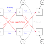 Understanding causal direction using the cross-lagged model
 Estimating change in time. Comparing the multilevel model for change with the Latent Growth Model