In a previous post we have seen how we can use multilevel modeling to understand change in time and how to separate within and between individual variation. Multilevel modeling is also the tool of choice in other research areas, such as educational or cross-national research. In this post I will give a short introduction of how to do cross-country analysis using multilevel modeling with the European Social Survey (ESS). You can download the data for free from: europeansocialsurvey.org.
Why use multilevel modeling?
In the social world we often have nested data. Some classical examples are: children nested in schools, individuals nested in households, individuals nested in countries, time nested within individuals (in longitudinal data).
These structures are important for two reasons. Firstly, classical regression modeling assumes that cases are independent. This is probably not true when we have such nesting. For example, pupils going at the same school probably have similar outcomes (or more similar than a random sample). Similarly, individuals from the same countries have some similarities due to shared language, culture, education, history and institutions. So, in these situations the assumptions of OLS regression are not met. Ignoring the nesting would lead to biased results. Multilevel modeling insures we get correct coefficients that account for the nesting in the data.
Secondly, this nesting actually can tell us important things about the social world. Knowing how much variation we have at each level can inform policies and theory. For example, it could tell us how important is culture in explaining people’s support for immigration. At one extreme you could have situations where everyone in a country has the same attitude to immigration. This would imply that culture is the only cause for our view of immigrants. At the other extreme all the variation could come from the individual, implying that culture has no role to play in our views of immigrants. Multilevel models allows us to estimate these different sources of variation.
Getting to know your data
We will be using a very small part of the ESS that has four variables:
- “id” (individual level ID)
- “cntry” (country, also acts as country level ID)
- “imbgeco” (“Immigration bad or good for country’s economy” – 0-10, larger = support for immigration)
- “eduyrs_cap” (years of education capped at 25)
We will be using the tidyverse package for data cleaning and visualization and lme4 for the multilevel modeling.
Let’s start by loading the package and having a look at the data:
# load package for data management and visualization
library(tidyverse)

# look at data
glimpse(ess)

## Rows: 34,056
## Columns: 4
## $ id         <int> 1, 2, 3, 4, 5, 6, 7, 8, 9, 10, 11, 12, 13, 14, 15, 16, 17, ~
## $ cntry      <chr> "AT", "AT", "AT", "AT", "AT", "AT", "AT", "AT", "AT", "AT",~
## $ imbgeco    <dbl+lbl>  5,  6,  5,  2,  5,  3,  5,  6,  6,  2,  2, 10,  6,  3,~
## $ eduyrs_cap <dbl> 12, 8, 11, 12, 12, 11, 8, 13, 12, 11, 13, 12, 12, 12, 8, 12~
When you do multilevel analysis you need to understand the nested structure of your data. Here we have individuals nested in countries. Before we do any fancy modeling we need to see how large are our samples:
# find out how many countries and cases we have
count(ess, cntry)

## # A tibble: 19 x 2
##    cntry     n
##    <chr> <int>
##  1 AT     2365
##  2 BE     1742
##  3 BG     1827
##  4 CH     1482
##  5 CY      761
##  6 CZ     2225
##  7 DE     2318
##  8 EE     1860
##  9 FI     1730
## 10 FR     1923
## 11 GB     2164
## 12 HU     1548
## 13 IE     2138
## 14 IT     2578
## 15 NL     1618
## 16 NO     1371
## 17 PL     1326
## 18 RS     1803
## 19 SI     1277
We see we have 19 countries and around 2000 people in each country. This should be enough for some multilevel models (opinions differ about the sample sizes needed to run these models).
Our outcome of interest is support for immigration. Before we do the model we should understand this variable and what kind of variation we have across countries. Bellow we do some descriptives by country where:
group_by()just does all the following functions by countrysummarise()creates summary statistics. The first two should be self-explanatory. In the last one we are checking if the cases are missing and then taking the average of that. This basically creates the proportion of missing casesmutate_if()just rounds all the numeric variables to 2 decimal points for ease of readingprint()just makes sure it prints all the rows
# explore our outcome variable
ess %>%
  group_by(cntry) %>%
  summarise(mean = mean(imbgeco, na.rm = T),
            SD = mean(imbgeco, na.rm = T),
            miss = mean(is.na(imbgeco))) %>%
  mutate_if(is.numeric, ~round(., 2)) %>%
  print(n = 50)

## # A tibble: 19 x 4
##    cntry  mean    SD  miss
##    <chr> <dbl> <dbl> <dbl>
##  1 AT     5.28  5.28     0
##  2 BE     5.3   5.3      0
##  3 BG     4.12  4.12     0
##  4 CH     6.17  6.17     0
##  5 CY     4.11  4.11     0
##  6 CZ     4.28  4.28     0
##  7 DE     6.13  6.13     0
##  8 EE     4.85  4.85     0
##  9 FI     5.72  5.72     0
## 10 FR     5.04  5.04     0
## 11 GB     5.89  5.89     0
## 12 HU     3.55  3.55     0
## 13 IE     6.11  6.11     0
## 14 IT     4.66  4.66     0
## 15 NL     5.55  5.55     0
## 16 NO     5.86  5.86     0
## 17 PL     5.69  5.69     0
## 18 RS     3.88  3.88     0
## 19 SI     4.46  4.46     0
We see that the average support for immigration and its variance differs quite a bit by country (indicating that MLM might be useful). We also see we don’t have any missing cases (I eliminated those in advance to make things easier).
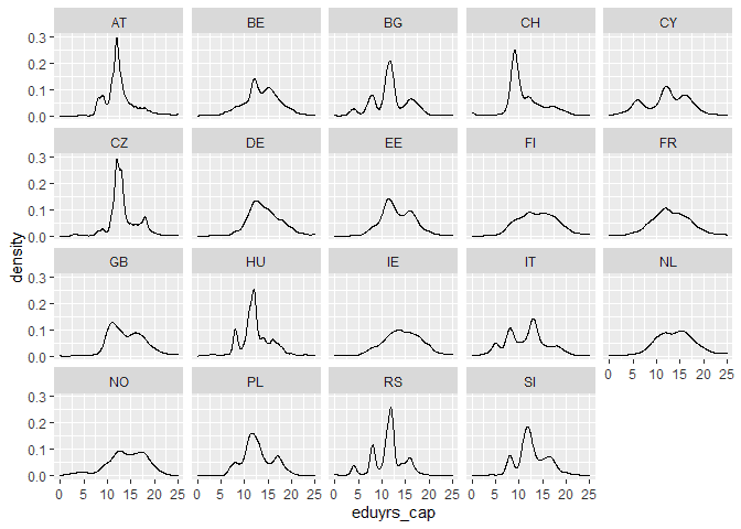
We can also check the distributions by country for the two variables of interest:
# look at distribution by country
ess %>%
  ggplot(aes(imbgeco)) +
  geom_density() +
  facet_wrap(~cntry)
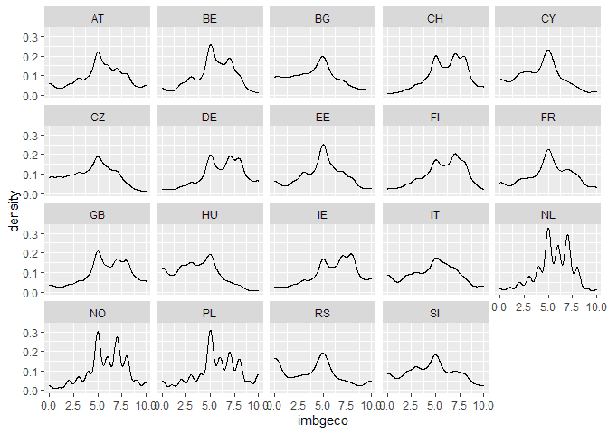
# look at education by country
ess %>%
  ggplot(aes(eduyrs_cap)) +
  geom_density() +
  facet_wrap(~cntry)
The multilevel model
In the multilevel model we separate sources of variation. In our case we want to separate individual and country level information so we have two different sources of variation. Typically, we want to start with a simple (empty or no predictors) model so we have a reference point and we can understand how much variation we have at each level. One way to write this is:
Yij = γ00 + U0j + Rij
Where
- Yij is the outcome or dependent variable (“imbgeco” in our case) that varies by individual, i, and country, j
- γ00 is the intercept, or the expected value of the outcome over all the individuals and countries (i.e., average)
- U0j is the between country variation. Tells us how different are the countries from each other on the outcome. If all the countries have the same average support for immigration this coefficient would be 0. If they are very different then this would be (relatively) large
- Rij is the residual of the regression, or in this case, the individual level variation. It tells us how different are the individuals from each other within each country. If everyone in a country would have the same value or if we can explain the outcome perfectly this would be 0.
We also assume these residuals are normally distributed, have a mean of 0 and a variance that has to be estimated:
U0j ∼ Normal(0, τ2)
Rij ∼ Normal(0, σ2)
Now that we got that out of the way let’s look at some real data. We will use the lmer() command from the lme4 package to run the multilevel models. The syntax is very similar to a normal regression in R except we put the random effects in a bracket where we have to say what coefficient varies by what variable. In our case we want to say that the intercept (represented by “1”) varies by “cntry”. We save the result as “m0” and then we print it using summary():
# load package for MLM
library(lme4)

# empty multilevel model
m0 <- lmer(imbgeco ~ 1 + (1 | cntry), data = ess)

# details of results
summary(m0)

## Linear mixed model fit by REML ['lmerMod']
## Formula: imbgeco ~ 1 + (1 | cntry)
##    Data: ess
##
## REML criterion at convergence: 156443.6
##
## Scaled residuals:
##      Min       1Q   Median       3Q      Max
## -2.56674 -0.64222  0.06111  0.71474  2.68192
##
## Random effects:
##  Groups   Name        Variance Std.Dev.
##  cntry    (Intercept) 0.6977   0.8353
##  Residual             5.7710   2.4023
## Number of obs: 34056, groups:  cntry, 19
##
## Fixed effects:
##             Estimate Std. Error t value
## (Intercept)   5.0884     0.1921   26.49
We see we have 34,056 cases and 19 groups. The coefficients of interest are:
- 5.0884 is the intercept or the expected value (i.e., average) of support for immigration in all the countries and individuals.
- 0.6977 is the country variation in support for immigration
- 5.7710 is the individual level variation in support for immigration
The random coefficients are hard to interpret on their own as the scale depends on the outcome. A solution to this is the ρ coefficient (also called the InterClass Correlation – ICC):
ρ = τ2/(τ2 + σ2)
This just measures the proportion of variation that is due to the countries out of the total amount of variation. In our case that would be:
# calculate ICC
0.6977/(5.771 + 0.6977)

## [1] 0.1078578
So it seems that around 10% of the variation in the support for immigration comes from the country in which you live (meaning also that 90% is due to individual characteristics). Another way to think about this is that if you randomly select two individuals from the same country the expected correlation in their support for immigration is 0.1.
To get an intuition about what country level and individual level variation mean we can have a look at this graph that shows just a few cases in three countries:
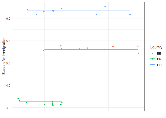
The country level variation comes from how different are the lines (average support for immigration) between countries. If this is very low then the lines will be very similar. If they are large, they will be very different. The individual level variation is a summary of the differences between each individual (dot) and their country line (e.g., distance from red dots to the red line).
So let’s see how we can make a graph like this based on our model for all the countries. First, we predict the scores based on our model (predict() command) and save it as a new variable in our data. Then we make a graph that shows a linear average line for each country (geom_smooth(se = F), method = lm estimates a linear trend without confidence intervals). Here we plot the prediction against years of education just for convenience and then we hide the x labels (this variable is not in the model so we expect a flat line).
# predict the scores based on the model
ess$m0 <- predict(m0)

# graph with predicted country level support for immigration
ess %>%
  ggplot(aes(eduyrs_cap, m0, color = cntry, group = cntry)) +
  geom_smooth(se = F, method = lm) +
  theme_bw() +
  theme(axis.text.x = element_blank(),
        axis.ticks = element_blank()) +
  labs(x = "", y = "Support for immigration", color = "Country")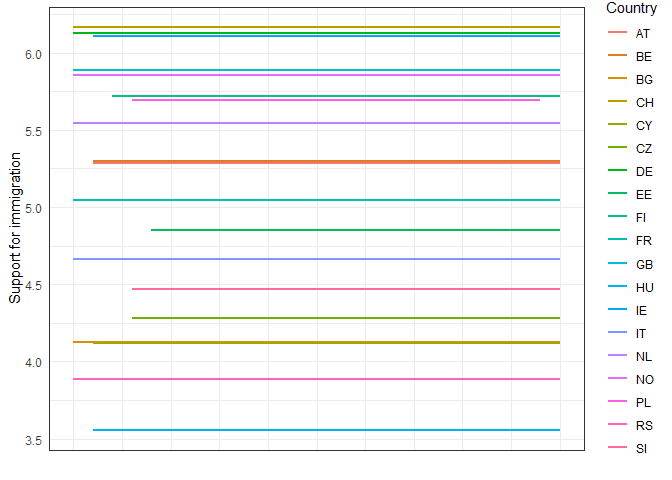
We see that this model allows each country to have a different average support for immigration through the random effect. We could visualize these random effects in a different way, using a dotplot (here I use the lattice package for convenience, it’s possible to do this in ggplot but slightly more code). We use the qqmath() command with the random effects from the model (extracted using ranef() command).
# dotplot using lattice package
library(lattice)
qqmath(ranef(m0, condVar = TRUE))
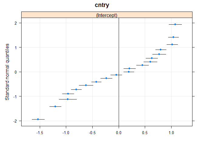
In this graph each dot represents a country and the line around it is the confidence interval. The 0 on the x axis is the intercept or expected value. So we see that most countries have values significantly different from that (confidence intervals do not include it), again indicating that this is a relevant level for the analysis.
Including predictors in MLM models
So far we only looked at an empty model but the main reason why we develop these models is to include predictors and understand relationships between independent variables and the outcomes.
We can easily develop the model like in a regular regression to include predictors. The interpretation is exactly the same:
Yij = γ00 + β1xij + U0j + Rij
So β1 is the expected change in the outcome when xij goes up by 1. Let’s see how this would look in our data if we wanted to explain support for immigration using education:
# random intercept with a control variable
m1 <- lmer(imbgeco ~ 1 + eduyrs_cap + (1 | cntry), data = ess)

# print results
summary(m1)

## Linear mixed model fit by REML ['lmerMod']
## Formula: imbgeco ~ 1 + eduyrs_cap + (1 | cntry)
##    Data: ess
##
## REML criterion at convergence: 155214.2
##
## Scaled residuals:
##     Min      1Q  Median      3Q     Max
## -3.1611 -0.6241  0.0685  0.6868  3.1725
##
## Random effects:
##  Groups   Name        Variance Std.Dev.
##  cntry    (Intercept) 0.5916   0.7692
##  Residual             5.5653   2.3591
## Number of obs: 34056, groups:  cntry, 19
##
## Fixed effects:
##             Estimate Std. Error t value
## (Intercept) 3.514725   0.182420   19.27
## eduyrs_cap  0.120730   0.003399   35.52
##
## Correlation of Fixed Effects:
##            (Intr)
## eduyrs_cap -0.243
Here we see that as years of education increases by 1 the expected support for immigration increases by 0.12. The intercept now is understood as the expected support for immigration when the independent variable is 0 (so for people without any years of schooling).
We also notice that the random effects are smaller compared to the previous model. This indicates that years of education is explaining some variation both at the individual and country level. We can visualize the relationship between the two variables as implied by our model using again predictions and a nice graph:
# save predicted scores
ess$m1 <- predict(m1)

# plot lines based on our model
ess %>%
  ggplot(aes(eduyrs_cap, m1, color = cntry, group = cntry)) +
  geom_smooth(se = F, method = lm) +
  theme_bw() +
  labs(x = "Years of eduction",
       y = "Support for immigration",
       color = "Country")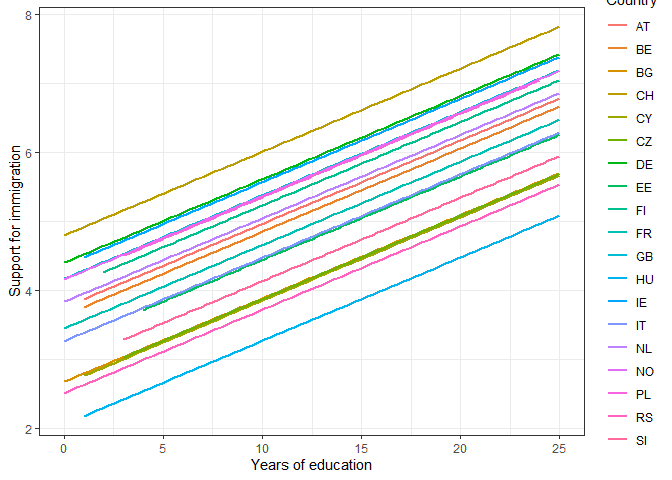
The random slope model
The previous model makes the assumption that the effect of education on attitudes to immigration is the same in all the countries (that’s why the lines are parallel). What if that is not the case? What if one year of education is more “effective” in some countries than others in raising the support for immigration.
This is where the random slope models come in. We can estimate a new coefficient that tells us how different are countries to each other in the effect of education on support for immigration. The model is:
Yij = γ00 + γ10xij + U0j + U1jxij + Rij
Where U1j is a new random effect (i.e., random slope) that summarizes the variation between countries in the effect of xij.
We can easily run such a model by including the education variable also in the random part of the model:
# model with random slope
m2 <- lmer(imbgeco ~ 1 + eduyrs_cap +
             (1 + eduyrs_cap | cntry),
           data = ess)

# print results
summary(m2)

## Linear mixed model fit by REML ['lmerMod']
## Formula: imbgeco ~ 1 + eduyrs_cap + (1 + eduyrs_cap | cntry)
##    Data: ess
##
## REML criterion at convergence: 155081.1
##
## Scaled residuals:
##     Min      1Q  Median      3Q     Max
## -3.1407 -0.6226  0.0633  0.6720  2.9673
##
## Random effects:
##  Groups   Name        Variance Std.Dev. Corr
##  cntry    (Intercept) 0.69715  0.83495
##           eduyrs_cap  0.00209  0.04571  -0.44
##  Residual             5.53696  2.35307
## Number of obs: 34056, groups:  cntry, 19
##
## Fixed effects:
##             Estimate Std. Error t value
## (Intercept)  3.51750    0.19740   17.82
## eduyrs_cap   0.11978    0.01106   10.83
##
## Correlation of Fixed Effects:
##            (Intr)
## eduyrs_cap -0.483
## optimizer (nloptwrap) convergence code: 0 (OK)
## Model failed to converge with max|grad| = 0.00804074 (tol = 0.002, component 1)
Ignore the convergence issue for now.
We see that now the fixed effect of education is slightly smaller and that we have a new coefficient in the random part of the model. The variance of the random slope for years of education is 0.00209.
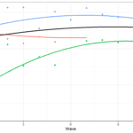
This coefficient is hard to interpret on its own. So let’s do another graph like before, based on the prediction from the model. This time we plot the average effect in a thicker blue line and all the country effects in thinner, slightly transparent lines:
# predict results based on our model
ess$m2 <- predict(m2)

# visualize the predictions based on our model
ess %>%
  ggplot(aes(eduyrs_cap, m2)) +
  geom_smooth(se = F, method = lm, size = 2) +
  stat_smooth(aes(color = cntry, group = cntry),
              geom = "line", alpha = 0.4, size = 1) +
  theme_bw() +
  guides(color = F) +
  labs(x = "Years of education",
       y = "Support for immigration",
       color = "Country")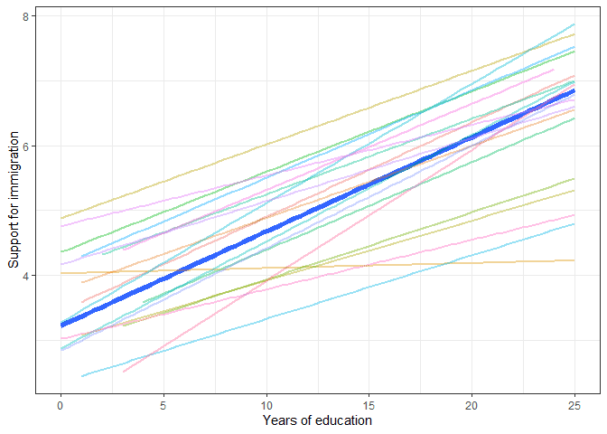
We see that there is a average effect that is represented by the fixed effect (0.11978) but each country is allowed to have its own line. In some countries education is more important for increasing support for immigration (steeper line) while in other countries the line is almost flat, indicating that education is not related to immigration support.
We can also visualize this using dotplots:
# another way to see random effect
qqmath(ranef(m2, condVar = TRUE))
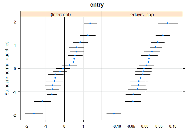
The new graph for “eduyrs_cap” shows how the effect of education on immigration support varies by country. We see that there are four countries on the top right where the effect of education is significantly more important while on the bottom left there are some countries where the effect is significantly lower.
To better understand where each country is positioned on these random effects we can create yet another graph. Here we plot the random effect for the intercept vs. the random effect for the slope for each country. We put a label with the names for each one for ease of reading and also a regression line to highlight the relationship between random intercepts and slopes:
# yet another way to look at the random effects

# save coefficients
coefs_m2 <- coef(m2)

# print random effects and best line
coefs_m2$cntry %>%
  mutate(cntry = rownames(coefs_m2$cntry))  %>%
  ggplot(aes(eduyrs_cap, `(Intercept)`, label = cntry)) +
  geom_point() +
  geom_smooth(se = F, method = lm) +
  geom_label(nudge_y = 0.15, alpha = 0.5) +
  theme_bw() +
  labs(x = "Slope", y = "Intercept")
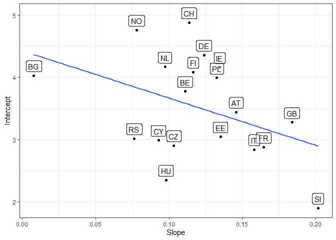
The graphs shows that some countries, for example Bulgaria (BG), have high average support for immigration but low effects of education on the outcome. Slovenia (SI), on the other hand has low average support for immigration but education has a stronger effect. In Great Britain (GB) there is average support for immigration but education has a strong effect on the outcome.
The blue line represents the relationship between the random intercept and slope. This is also presented in the results and is -0.44 in this case. This would indicate that the less average support for immigration in a country the more important individual level education becomes (although we need to be careful with that interpretation given the small number of countries and the strange behavior of Bulgaria).
Conclusions
Hopefully this will get you started with using R and multilevel modeling in cross-national research. We saw just some basic models but we covered some essential concepts like random intercept, random slope and ICC. If you want to see how you can apply multilevel modeling to longitudinal data you can check out this blog post. If you liked this you can have a look at the training that I offer.
If that was useful you might also like the Longitudinal Data Analysis Using R book.
This covers everything you need to work with longitudinal data. It introduces the key concepts related to longitudinal data, the basics of R and regression. It also shows using real data how to prepare, explore and visualize longitudinal data. In addition, it discusses in depth popular statistical models such as the multilevel model for change, the latent growth model and the cross-lagged model.
More blog posts
 Estimating non-linear change in time using the multilevel model for change
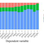 Measurement error in health data collection. The case for nurse effects
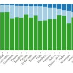 How do interviewers influence the study of discrimination?
 #freesurveydata: European Values Study 2017 (Updated 2019)
 Call for abstracts 4th Mobile Apps and Sensors in Surveys workshop
 Survey methods deadlines and events: March 2019
Thank you for this article. You summarise HLM in R neatly.